Management & Decision Sciences
Cutting Edge (Nova Southeastern)
Part 1
Mark Lawrence has been pursuing a vision for more than two years. This pursuit began when he became frustrated in his role as director of Human Resources at Cutting Edge, a large company manufacturing computers and computer peripherals. At that time the Human Resources Department under his direction provided records and benefits administration to the 60,000 Cutting Edge employees throughout the United States, and 35 separate records and benefits administration centers existed across the country. Employees contact these records and benefits centers to obtain information about dental plans and stock options, change tax forms and personal information, and process leaves of absence and retirements. The decentralization of these administration centers caused numerous headaches for Mark. He had to deal with employee complaints often since each center interpreted company policies differently – communicating inconsistent and sometimes inaccurate answers to employees. His department also suffered high operating costs since operating 35 separate centers created inefficiency.
His vision? To centralize records and benefits administration by establishing one administration center. This centralized records and benefits administration center would perform two distinct functions: data management and customer service. The data management function would include updating employee records after performance reviews and maintaining the human resource management system. The customer service function would include establishing a call center to answer employee questions concerning records and benefits and to process records and benefits changes over the phone.
One year after proposing his vision to management, Mark received the go-ahead from Cutting Edge corporate headquarters. He prepared his “to do” list – specifying computer and phone systems requirements, installing hardware and software, integrating data from the 35 separate administration centers, standardizing record-keeping and response procedures, and staffing the administration center. Mark delegated the systems requirements, installation, and integration jobs to a competent group of technology specialists. He took on the responsibility of standardizing procedures and staffing the administration center.
Mark had spent many years in human resources and therefore had little problem with standardizing record-keeping and response procedures. He encountered trouble in determining the number of
This case was adapted from Hiller, Frederick S. & Mark S. Hillier (2014). Introduction to Management Science: A Modeling and Case Studies Approach with Spreadsheets, 5th ed., McGraw-Hill/Irwin, pp 429-432.
2
representatives needed to staff the center, however. He was particularly worried about staffing the call center since the representatives answering phones interact directly with customers – the 60,000 Cutting Edge employees. The customer service representatives would receive extensive training so that they would know the records and benefits policies backwards and forwards – enabling them to answer questions accurately and process changes efficiently. Overstaffing would cause Mark to suffer the high costs of training unneeded representatives and paying the surplus representatives the high salaries that go along with such an intense job. Understaffing would cause Mark to continue to suffer the headaches from customer complaints – something he definitely wanted to avoid.
The number of customer service representatives Mark needed to hire depended on the number of calls that the records and benefits call center would receive. Mark therefore needed to forecast the number of calls that the new centralized center would receive. He approached the forecasting problem by using judgmental forecasting. He studied data from one of the 35 decentralized administration centers and learned that the decentralized center had serviced 15,000 customers and had received 2,000 calls per month. He concluded that since the new centralized center would service four times the number of customers – 60,000 customers – it would receive four times the number of calls – 8,000 calls per month.
Mark slowly checked off the items on his “to do” list, and the centralized records and benefits center opened one year after Mark had received the go-ahead from corporate headquarters.
Now, after operating the new center for 13 weeks, Mark’s call center forecasts are proving to be terribly inaccurate. The number of calls the center receives is roughly three times as large as the 8,000 calls per month that Mark had forecasted. Because of demand overload, the call center is slowly going to hell in a handbasket. Customers calling the center must wait an average of five minutes before speaking to a representative, and Mark is receiving numerous complaints. At the same time, the customer service representatives are unhappy and on the verge of quitting because of the stress created by the demand overload. Even corporate headquarters has become aware of the staff and service inadequacies, and executives have been breathing down Mark’s neck demanding improvements.
Part 2
Mark needed help, and he approached Harry, a corporate analyst, to forecast demand for the call center more accurately.
Luckily, when Mark first established the call center, he realized the importance of keeping operational data, and he provided Harry with the number of calls received on each day of the week over the last 13 weeks. The data (refer to Cutting Edge Student File No. 1) begins in week 44 of the last year (2012) and continues to week 5 of the current year (2013).
Mark indicates that the days where no calls were received were holidays.
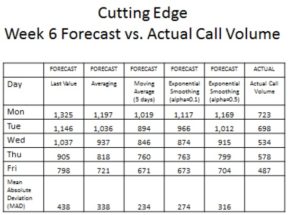
As a start, Harry used the data from the past 13 weeks and applied five different time-series forecasting methods in preparing a trial forecast of the call volume for each day of the upcoming week (Week 6). He provided a different forecast for each day of the week by treating the forecast for a single day as being the actual call volume on that day.
From plotting the data, Harry could see that demand follows “seasonal” patterns within the week. For example, more employees call at the beginning of the week when they are fresh and productive than at the end of the week when they are planning for the weekend. Therefore, Mark prepared and used seasonally adjusted call volumes for the past 13 weeks. After Week 6 ended, Harry compared the five forecasts with the actual volumes and calculated the Mean Absolute Deviation (MAD) values for each method. The result of Harry’s work is summarized below:
Part 3
After many months of work and with Harry’s help, Mark has been able to stabilize the call center operation. Mark now has a better handle on how to forecast the daily call demand and he is able to prepare effective weekly staffing schedules for handling the daily variation in volume.
However, Mark is still experiencing difficulty in forecasting the volume from month to month. Cutting Edge has been very active in acquiring new companies while, at the same time, selling off portions of their existing business. Mark believes that this activity is causing fluctuations in call volume because it is affecting the employee head count of Cutting Edge.
Mark has assembled monthly data for call volume and head count for the past 18 months (refer to Cutting Edge Student File No. 2). Mark also suspects that there are other factors which may be affecting the call volume, and he has noted these factors on the attached spreadsheet. Based on the upcoming acquisition of Cutter Corp on 7/1/2015, the forecast of head count for July 2015 is 77,000.
Individual Case Study Report
Winter 2017[1]
The Prescott Bakery Company Case Study
Qnt. 5160
Maximum Points: 25
There are three parts to this individual case study be sure that you answer each part completely. You may answer these questions directly into this Word document. When you save it, save it as the following: (Your last name) Individual Case Study. Submit it into the Blackboard drop box by the deadline listed in your class calendar. You must have, as the front page, the required NSU/CBE front page with your typed signature attesting that you have not copied answers.
Hints are provided throughout this document. It is strongly suggested that you follow those hints to obtain the maximum number of points in this important exercise. Read the backstory carefully, it will explain much of the information that you need to understand about this case study. Remember to write this report directly to William Flours whom you will meet in just a few minutes. Bill is NOT a statistician and does not understand much about these forecasting techniques, so explain them to him in a way that he will understand. Completely explain terms and concepts when they first appear in the case study questions. You need not explain the same term more than once, but explain each one completely so that Bill can understand it.
There are two Excel spreadsheets (blank) that are needed for part 3. They are the Exponential Smoothing Spreadsheet, and the Blank Linear Regression Spreadsheet. Your professor has explained how to use them in your weekly chats, so refer to them or ask questions if you are lost. Now on to our story.
The Prescott Bakery Company Story
The Prescott Bakery Company is an old line company started in Prescott, Florida by the Flours family right after the Civil War. The company has moved as it expanded, with the latest bakery located just east of town off of State Route 13, about 2 miles out of Prescott. The current company president, William (Bill) Flours is an energetic man who loves baking and has said that “If I cut myself, I guess I’d bleed flour”. His daughter, Robin, has been groomed to take over the company when her dad retires in about 10 years. Until then she is taking graduate business classes at Florida Northwestern State which is about 90 miles northwest of Prescott.
Robin is concerned that her dad does not do much to forecast production, and said recently “He seems to fly by the seat of his pants”. She has been working with him to get a forecasting method for the company’s pies. While the bakery is a full service company, producing breads, rolls, and other bakery products, it is well known for its pies. In fact, the company sponsors one of the biggest festivals in Prescott, the Fall Pie Spectacular. Thousands of people flock into town one weekend in July when “pies rule”. So Robin has been working on a number of forecasting techniques to try and solve the problem of how many pies should the bakery produce each month.
The bakery produces about 5,000 pies a month selling them for between $5.00 to a little over $7.00 a pie. The type of pie determines the price, but we will not be concerned with the type of pie in this case study, just in the amount of pies that the company should produce during January 2017. We have information about their production for the entire year of 2016, but Robin is working toward showing her father that using the correct forecasting technique he can estimate his production for any month.
Later in this case study you will be combining the cost of the pies and the number produced to come up with a production schedule, but for right now you will be concentrating on the number of pies for the month of January[2]. The production for the entire year is found below. Review it before you attempt this case study.
| Prescott Bakery Pie Production 2016[3] |
| |
January |
4,870 |
$6.25 |
| |
February |
4,965 |
$5.95 |
| |
March |
4,915 |
$5.50 |
| |
April |
5,107 |
$6.15 |
| |
May |
5,048 |
$7.29 |
| |
June |
5,102 |
$6.99 |
| |
July |
5,146 |
$6.39 |
| |
August |
4,965 |
$6.69 |
| |
September |
5,040 |
$6.45 |
| |
October |
4,968 |
$7.10 |
| |
November |
5,065 |
$6.85 |
| |
December |
5,019 |
$6.99 |
|
|
|
|
Robin is off at school right now and has asked you, her close friend, to help with a preliminary report on various forecasting techniques and concepts. So this is your chance to help her, and make a few dollars in return for your efforts[4]. Remember, her dad does not understand statistics, so whatever you explain, be sure that he can understand it, and that your description is complete.
Part 1.
The Forecasting Techniques
Robin has tried out a number of techniques that she thinks will work well at the bakery. While she knows that there are other forecasting techniques (she has a very competent statistics professor at FLNWS), but she wants to keep the techniques simple and easy to understand.
Robin needs to help her dad go through the various forecasting planning steps, but she has not done this yet, so you will have to help her.[5]
Based on the five (5) steps in creating a forecast, help Bill Flours by presenting him with suggestions that walk him through each of these steps. Remember, Bill is not a statistician, so help him with common English terms, (and define any uncommon ones) and go through each of these steps with him so that he can understand what they mean.
Step 1: Define the Problem to be solved
Step 2: Gather Statistical and Other Data
Step 3: Look for Patterns in the Data or Outliers
Step 4: Select a Forecasting Model to Use[6]
Step 5: Evaluate the Results of the Forecasting Model and Apply the Results
Part 2.
On her last vacation Robin used five different techniques to show her dad how this forecasting works. Your first job will be to explain these techniques to her dad.
| Prescott Bakery Pie Forecasting Summary |
|
|
|
| |
|
|
Forecasting technique |
|
|
| Statistic |
Last Value |
Averaging |
Moving Average 3MA |
Exponential Smoothing with Seasonality (a=.1) |
Exponential Smoothing with Seasonality (a=.5) |
| MAD |
129 |
126 |
136 |
88 |
70 |
| MSE |
26,046 |
24,989 |
26,314 |
10,504 |
7,512 |
| January Forecast |
5,019 |
5,129 |
5,181 |
5,134 |
5,026 |
For each of these techniques explain (1) what the technique is, (2) how does it work and then (3) what the results mean. You only need to explain the MAD and the MSE once, but make sure that Bill can understand what you are telling him, then at the end of this section compare and contrast these different forecasting techniques and recommend that he consider adopting one (and only one) to use as a possible forecasting technique. Be sure to explain your reasons for this decision. Type your responses in the following section, but remember to explain these results completely within each section.
- The Last Value Forecasting Technique
- The Averaging Forecasting Technique
- The Moving Average Forecasting Technique (3MA)
- The Exponential Smoothing Forecasting Technique with alpha = .1
- The Exponential Smoothing Forecasting Technique with alpha = .5
- Recommendation on which Forecasting Technique to Select and Why
Part 3 – Casual Forecasting versus Exponential Smoothing
In this third part you will be using two Excel templates to calculate both a linear regression and an exponential smoothing and then compare and contrast the two. You must explain your decision either way.
Using the two Excel files provided to you, the Blank Linear Regression Spreadsheet and the Exponential Smoothing Spreadsheet to prepare several forecasts using the raw data as seen below. There are 2 columns of data, the middle column[7] is used for the Exponential Smoothing, and both the left and middle columns[8] are used for the linear regression. The month column is not needed for either of these calculations.
The Raw Data
| Prescott Bakery Pie Production 2016 |
| Month |
Pies Produced |
Average Selling Price |
| January |
4,870 |
$6.25 |
| February |
4,965 |
$5.95 |
| March |
4,915 |
$5.50 |
| April |
5,107 |
$6.15 |
| May |
5,048 |
$7.29 |
| June |
5,102 |
$6.99 |
| July |
5,146 |
$6.39 |
| August |
4,965 |
$6.69 |
| September |
5,040 |
$6.45 |
| October |
4,968 |
$7.10 |
| November |
5,065 |
$6.85 |
| December |
5,019 |
$6.99 |
Exponential Smoothing
Using the Exponential Smoothing Spreadsheet, import the raw data on the number of pies produced during 2016, set the Initial Estimate Average to 5,000. First set alpha at .1, then at .5, and then again lastly at .9 and complete the following table with the output information from the spreadsheet.
Exponential Smoothing Results
| Forecast Output |
Alpha = .1 |
Alpha = .5 |
Alpha = .9 |
| MAD |
|
|
|
| MSE |
|
|
|
| January Forecast |
|
|
|
NOTE: You may have to copy the Exponential Smoothing Forecast to the next blank space below to create the forecast for the month of January.
After you have completed this, then compare and analyze the results including the three graphs that are produced as you change the alpha. In short, you will see three different results as you change the alpha. Answer these questions:
- What is the difference in the smoothing of the data as you change the alpha values? Explain completely.
- How do the MAD and MSE change as you change the alpha values? Explain completely why you think this is happening.
- Of these three different forecasting options, which one appears to produce the best forecast and why?
The Causal Forecasting Technique
Using the linear regression spreadsheet and using the monthly pie production as the dependent variable and the cost per pie as the independent variable, change the Estimator to 5,000 and complete the following table.
Linear Regression Results
| Estimated Error |
Cost per Pies |
Estimated number of Pies Produced |
| |
$6.50 |
|
| |
$7.00 |
|
| |
$7.50 |
|
NOTE: If you have forgotten how to use the results of the linear regression go to the PowerPoint presentation for week 5, slide 54 for how to do these calculations.
Answer the following questions about the linear regression.
- Which of these pie costs yield the most pies produced and why?
- Which of these pie costs yield the least pies produced and why?
Summary Section
Comparing only the causal forecasting technique and the Exponential techniques (Part 3 only) which of these techniques would you recommend to Bill to use as a production forecasting technique, and why?
This concludes this individual case study. Be sure to post it as well as a copy of both the linear and exponential smoothing spreadsheets into the Blackboard Dropbox by the deadline for your class.
#
[1] While your professor reuses the basic information for these case studies, the data changes each term. Do NOT make the mistake of copying results from a prior term, or you will earn ZERO points for copying.
[2] By the way, this month has already passed and Robin knows the actual production for the month of January, but she wants to prove to her dad that forecasting works, so after this is all over she will review the actual production with the forecasted production with him.
[3] While this case study shell has been used before, the data has been changed, so don’t cheat and use prior data, it will be WRONG.
[4] She has offered you $1,500 to help her, so make it a good report.
[5] Remember you learned these planning techniques way back in Week 4, slides 9 through 14. Go there to refresh your memory as to what is required to accomplish in this planning.
[6] Here you may discuss in general what are common forecasting techniques.
[7] The number of pies produced by month.
[8] The cost of each pie sold.
Which of the following statements about Big Data is true?
Why are analytical decision making skills now viewed as more important than interpersonal skills for an organization’s manager?
The HP Case study illustrate that after analytics are chosen to solve a problem, building new decision model from scratch or purchasing one may not always be the best decision approach. Why is that?
Business Intelligence (BI) can be characterized as a transformation of ……… data to information to decisions to action
How are descriptive analytics different from the other two types?
Question 1
- The number 5.6E-05 appears in a cell. Which one of the following statements is correct?
|
|
the actual number is 560,000 |
|
|
the actual number is 0.6 |
|
|
the actual number is 5.55 |
|
|
the actual number is 0.000056 |
|
|
there is a calculation error in the cell |
Question 2
- You wish to calculate the square root of the value in cell D4 in an Excel spreadsheet. Which of the following would NOT give the correct answer?
|
|
=D4^(1/2) |
|
|
=SQRT(D4) |
|
|
=ROOT(D4) |
|
|
=D4^0.5 |
|
|
=EXP(LN(D4)/2) |
Question 3
- Which of the following is a legitimate statistical function in Excel:
|
|
=RANGE(E2:E93) |
|
|
=ZSCORE(E2:E93) |
|
|
=VARIANCE(E2:E93) |
|
|
=MEAN(E2:E93) |
|
|
=AVERAGE(E2:E93) |
Question 4
- In order to invoke the “go to” dialog box in Excel so as to move the cursor to a specific cell, press:
1 points
Question 5
- The cells C1:C6 in a worksheet are being used in formulas in other cells. In order to make these cells absolutely referenced in row, enter the cells range and then press:
|
|
F4 once |
|
|
F4 twice |
|
|
F4 three times |
|
|
Ctrl plus F4 |
|
|
Alt plus F4 |
Question 6
- The distribution of the tenure data is best described as being:
|
|
excessively kurtotic |
|
|
excessively skewed |
|
|
visually approximately normal |
|
|
right skewed leptokurtic |
|
|
negatively skewed and platykurtic |
Question 7
- Which of the following statements about the sample is INCORRECT:
|
|
the mode is 69 |
|
|
50th percentile is 65 |
|
|
the mean is 60.32 |
|
|
the mean is 394.55 |
|
|
the mean < median < mode |
Question 8
- The variability of the sample is measured as:
|
|
a skewness of -0.77 |
|
|
a variance of 15.12 |
|
|
a coefficient of variation of 25% |
|
|
a standard deviation of 3349 |
|
|
a range of 21 |
1 points
Question 9
- Which of the following statements about the sample is correct:
|
|
the skewness is -0.77 |
|
|
the excess skewness is -0.28 |
|
|
the skewness is 10 |
|
|
the kurtosis is 10 |
|
|
the excess kurtosis is 100 |
1 points
Question 10
- “From the histogram or ogive (cumulative frequency chart) of the sample, which of the following statements is correct:”
|
|
the 40th percentile is 62 |
|
|
the 100th percentile is greater than 85 |
|
|
median is in the range 36-49 |
|
|
the median is in the range 49-62 |
|
|
the mean is 60.32 |
Performance Lawn Equipment
This problem was taken from Evans, J.R. (2013). Business Analytics: Methods. Models, and Decisions, 1st ed., NJ: Pearson Education, Inc., p. 84
Part 1. Performance Lawn Equipment (PLE) originally produced lawn mowers, but a significant portion of sales volume over recent years, has come from the growing small-tractor market. PLE sells their products world-wide, with sales regions including North America, South America, Europe, and the Pacific Rim. Three years ago a new region was opened to serve China, where a booming market for small tractors has been established. PLE has always emphasized quality and considers the quality it builds into its products as its primary selling point. In the past 2 years, PLE has also emphasized the ease of use of their products.
Before digging into the details of operations, Elizabeth Burke wants to gain an overview of PLE’s overall business performance and market position by examining the information provided in the database. Specifically, she is asking you to construct appropriate charts for the data in the following worksheets and summarize your conclusions from analysis of these charts:
- Dealer Satisfaction
- End-User Satisfaction
- Complaints
- Mower Unit Sales
- Tractor Unit Sales
- On-time Delivery
- Defects After Delivery
- Response Time
Part 2. The supply chain worksheets provide cost data associated with logistics between existing plants and customers as well as proposed new plants. Ms. Burke wants you to extract the records associated with the unit shipping costs of proposed plant locations and compare the costs of existing locations against those of the proposed locations using quartiles.
Part 3. Ms. Burke would also like a quantitative summary of the average responses for each of the customer attributes in the worksheet 2012 Customer Survey for each market region as a cross-tabulation (see Sample Table A) and as a histogram.
We can assist you in understanding course assignments using the following
Palisade Software@
The
DecisionTools
Suite
Complete @RISK and Decision Analysis Toolkit
@RISK
Risk analysis software using Monte Carlo simulation for Excel and Project
PrecisionTree
Decision trees for Microsoft Excel
StatTools
Advanced statistics toolkit
for Microsoft Excel
The Prescott county mayor, Robert (Pete) Smith has been worried for some time that housing values in the county have been declining. Pete said to the county commission recently,
“Our housing stock is getting so old and tired, and I’m afraid that if we don’t start building new homes that our children will just move away to Orlando or even to, heaven forbid, to South Florida. I think that we need to study this situation, and do something about it right now!”
What Pete did not say, but each of the commissioners knew, was that his brother-in-law, Bo Bradley is a developer who wants the commission to rezone 350 acres in the north county for a new development. This land is currently envisioned to be a county park, but old Bo want to develop it. Bo said recently, “What this county needs is my development, not some old park for the deer.” Bo it seems is interested in making money more than he is in protecting undeveloped land.
In order to get this study going Pete has asked you to look at some recent sales of homes in the county to understand what is going on with the housing stock, and then to project out what kind of values that five typical housing could bring. What he is hoping is that the values will be so low that the commission will want to rezone those 350 acres for Bo’s development.
Using the Excel data file that has been provided you are to completely answer the following questions:
1. What is the current status of the housing stock in the county?
a. To do this you will create a one-variable summary using StatTools and analyze the age of the recently sold homes, their average price sold, the number of bedrooms, bathrooms and number of cars that can be garaged.
b. What does the skewness and kurtosis tell you about these data?
c. Would it be better to use the Interquartile range to analyze this data (not a yes or no answer) and if so why, or why not?
2. Doing two Q-Q plots, do you consider the data for price and square footage to be normal or not, and why?
3. Doing a correlation in StatTools and using all six of the variables, how are each of these variables correlated to each other. Again be specific.
4. Doing a scatterplot of price versus square footage and adding a trend line to the plot, what does this tell you about the data?
a. Now do a scatterplot of price versus age and adding a trend line, what does this tell you about the question of new homes versus price?
5. Next do a multiple regression using price as the dependent variable, and all other variables as independent variables:
a. Do any of the variables have a t-value that is greater than the alpha (.05) for this assignment? If so, delete them and rerun the regression and compare and contrast the old regression versus the new regression without one or more of the variables.
b. Is the F-ratio for this/these regressions significant? Why?
c. Is the r-squared values for this/these regressions appear to be valid? Does it show that it explained a sufficient amount of the total variation?
6. Using the coefficients from this regression estimate the selling prices for the following typical Prescott county homes:
Home
number Square footage Age of the home Number of bedrooms Number of bathrooms Size of the garage (cars) Projected Selling Price (determined by you)
1 1,850 25 3 2 1
2 2,200 14 4 3 2
3 3,000 5 5 4 3
4 3,400 5 5 5 3
5 2,200 40 3 2 1
7. Based on the projected selling price of these homes, will Mayor Pete convince the county commission to rezone the land for his brother-in-law, or does the county get a new park? Defend your answer based on the statistics that you have calculated in this case study. Your argument should be no more than 300 words.
You are to do the following tests including explaining/analyzing the results of these statistical tests:
1. A one variable summary for all variables (single output with all variables on it).
2. A scatterplot with the price versus square footage, add a trend line and show the R2 value on the plot.
3. A correlation coefficient showing all variables – analyze the results.
4. Histograms for all variables – 6 different histograms.
5. A multiple regression with all 6 coefficients calculated correctly. Explain the r-squared value, what it means, the F-value and what it means, and the T-test values and what they mean.
a. Are there any variables that could be deleted from the regression? If there are rerun the regression without this variable(s).
b. If you remove one or more variable then recalculate the regression.
6. Predict the home selling price complete and include Table One found below in your written report:
Home
number
Square footage
Age of the home
Number of bedrooms
Number of bathrooms
Size of the garage (cars)
Projected Selling Price (determined by you)
| Price |
Sq. Feet |
Age |
Bedrooms |
Bathrooms |
Garage _ |
| 110000 |
1000 |
28 |
3 |
1 |
1 |
| 133500 |
1400 |
23 |
3 |
1 |
1 |
| 112500 |
1248 |
58 |
3 |
4 |
1 |
| 141750 |
1106 |
12 |
2 |
1 |
1 |
| 195250 |
2112 |
78 |
2 |
6 |
2 |
| 132250 |
1078 |
33 |
2 |
1 |
1 |
| 136000 |
952 |
13 |
2 |
3 |
2 |
This case was prepared by David Hoyte, Tom Griffin, and Yuliya Yurova, professors of Research Methods and Decision Sciences at the H. Wayne Huizenga School of Business and Entrepreneurship, Nova Southeastern University. It is intended as a basis for class discussion. Main characters, locations, and numbers in this case were modified to preserve privacy. Copyright (c) 2014, Nova Southeastern University. March. 31, 2014
Paws Palace Clinic has been a successful and growing veterinary practice in Parkland,Florida, owned and run by Veterinarian Dr. Bill Schulke, and his office manager / spouse, Sue Schulke. Over the last 12 months, the practice has been averaging $80 profit per patient visit, which is helpful for the young couple to pay back Bill’s enormous college loans. For the first two years of operation normal office hours at the clinic from 8:00am to 5:30pm.
Review @Risk interactive tutorial “@Risk Quick Start”. (To do this, open @Risk and go to Help; select Welcome to @Risk; a new window will open where you should select Quick Start to see the tutorial.)
Study the case “Paw Palace Pet Clinic” and download data file “Paw Palace Data.xlsx” from BB9. Compute descriptive statistics for historic inter-arrival and service times in tab Data. In @Risk, fit Normal, Uniform, Exponential, and Triangular distributions to historic inter-arrival and service times (IAT and ST). What is the best and what is the worst fitting distribution for IAT? For ST? Paste the @RISK histograms you develop for the IAT and ST (service time) data on your tab Data – input data worksheet.
Analyze the simulation model in tab “Current Model B”. Answer the following questions:
1. How many patients per day does the clinic serve on average? There is a 95% probability that _______ or more clients will be served per day.
2. What are the average daily and annual profits from the business? There is a 95% chance that $________ or more profit will be made per day; and $__________ or more will be made during the first year.
3. What are the average and maximum wait times? There is a _______% chance that customers will have to wait 25 minutes or less, a ________% chance that customers will have to wait between 20 and 40 minutes, and a ________% chance that customers will have to wait longer than 40 minutes.
4. What is the average number of reneges? There is a 95% chance that at least _____ of customers will renege daily. There is a 65% chance that no more than _____ customers will renege daily.
Prepare a report including Background, Problem Statement, Analysis (method of analysis, input variables, description of input variables). Do not submit your report.
Complete the simulation model for Paw Palace Pet Clinic to access the economic benefits to be obtained by hiring a veterinarian assistant:
Complete the formulas for waiting times and annual profit for a model with vet assistant in tab “Current and New Model C”. In @Risk, use Triangular distribution to simulate service times. Use 5, 15, and 35 minutes respectively as parameters.
Compute the change in annual profit to be obtained by hiring a veterinarian assistant. Designate the change in annual profit as an output in @Risk
Obtain distribution of the change in profit using 5000 iterations
Answer the following questions:
1. If Dr. Shulke were to hire vet assistant, hence, improving service time, how do outputs “1” – “4” in above (Assignment Week 3) change?
2. Analyze the distribution of the change in profit in terms of expected profit and risk (Hint: use percentiles and median).
3. What would customers perceive regarding wait times above, compared to before the new hire? Would the clinic be able to improve customer retention and grow business? Discuss pros and cons of hiring vet assistant.
This case was prepared by Mike Bendixen, professor of Research Methods and Decision Sciences at the H. Wayne Huizenga School of Business and Entrepreneurship, Nova Southeastern University. It is intended as a basis for class discussion rather than to illustrate effective or ineffective handling of an administrative situation. The numbers and characters in the case are fictitious. Copyright © 2013, Nova Southeastern University. December 1, 2013.
|
|
Saturday Scheduling at Eterno
“Where are you when I need you Jenna! Why do I have to work with idiots?” thought Alejandra as she sat down at her desk in frustration. Alejandra headed the workforce planning team for the inbound call center operations at Eterno Life. She had just returned from her first meeting with the Jeremy, the acting Service Executive, of Eterno Life and Alejandra’s boss while Jenna, her regular boss, was on four months maternity leave. Jeremy was a senior member of the Compliance Officer’s team and had been seconded a few days earlier to look after service operations while Jenna was away. Jeremy was regarded by many in call center as an obnoxious character with strong opinions and poor listening skills. She knew that the current problem that she was working on was going to take all her persuasive skills.
Eterno Life was a medium-sized life insurance company based in Modesto, CA. It had been started some 20 years ago by a smart young actuary, Gustavo Lopez, who was bored with working in the loss assessment office of one of the nation’s largest life insurance companies. Gustavo had always dreamed of running his own business and had carefully saved as much of his salary and bonuses for the day when the opportunity arose. When the father of one of his college friends had died in tragic circumstances leaving his family virtually destitute, Gustavo saw his opportunity. He started Enterno Life which offered simple and affordable life insurance and funeral coverage policies. The product line appealed to the large number of agricultural workers in the San Joaquin Valley, as did the high levels of service quality offered.
The main operating hours for the call center were from 7:00am to 7:00pm, Mondays to Fridays except for public holidays. At the special request of brokers, a small team handled calls on a Saturday morning from 9:00am to 12:00pm. The basis of this request was the high level of policy sales on Fridays, especially Friday evenings. In keeping with the service orientation of Enterno Life, this was agreed to some three years ago. Both brokers and customers were very happy with this service and it had even been featured in some of the company’s promotional material and advertisements.
Alejandra had noticed that service levels for this Saturday service were regularly not achieved and was about to suggest that the staff complement for this three hour shift be increased from three to four customer service representatives (CSRs). Eterno Life had established a shift target that 80% of calls should be answered within 30 seconds and that no more than 10% of customers had to wait for their call to be answered. The Saturday shift regularly missed these target metrics.
Alejandra set up a meeting with Jeremy to approve this change. She had barely finished stating her case when Jeremy launched into a tirade claiming that, if anything, the staff complement should be reduced from three to two rather than increased to four. He argued that with three CSRs there was considerable idle time (when CSRs we not handling calls) so they were clearly goofing off and not getting their work done. Alejandra knew that this was not the case as she was regularly at work on Saturday morning to add the final touched to the staff schedules for the coming week. Her workspace was adjacent to the call center. Before she could defend her request, Jeremy tasked her with investigating the situation to justify the reduction in staffing and summarily ended the meeting, demanding a report within two days.
When she had calmed down, Alejandra set to gathering the data and start the analysis. Firstly, she extracted details of all the calls taken on the past four Saturdays. She noted that there were a total of 320 calls and calculated that the mean time between calls was 2.25 minutes (4 shifts x 3 hours/shift x 60 minutes/hour divided by 320 calls}. She knew that the time between calls followed an exponential distribution so that was relatively easy to model.
The handle time (customer talk time plus administrative wrap-up time after the call was completed) for the 320 calls is presented in the attached Excel spreadsheet. The mean handle time of this sample was 3.80 minutes which corresponded well with the standard of 3.83 minutes used for weekday shifts. However, in order to model the Saturday shift, it would be necessary to understand the distribution of these handle times. Alejandra remembered from her studies that service times generally followed a gamma distribution. This distribution has two parameters, shape and scale. However, the gamma distribution was difficult to work with and it would be preferable to use one of the special cases of this distribution: either the exponential distribution (shape parameter = 1) or the Erlang distribution (shape parameter = positive integer greater than one). The exponential distribution seemed an unlikely candidate as it has a mode of zero implying that the most frequently occurring situation would be calls with a zero handle time! As a last resort, a triangular distribution could be used to fit the data.
Lastly, Alejandra recalled that the formula for the percentage occupancy of a call center was given by:
100 X mean handle time/(mean time between calls x number of CSRs).
The percentage idle time was simply this number subtracted from 100.
With this, Alejandra started to model the Saturday shifts so as to write a report arguing for increasing the number of CSRs for the Saturday shift to four rather than reducing it to two.
Complete the simulation model for Paw Palace Pet Clinic to access the economic benefits to be obtained by hiring a veterinarian assistant:
Complete the formulas for waiting times and annual profit for a model with vet assistant in tab “Current and New Model C”. In @Risk, use Triangular distribution to simulate service times. Use 5, 15, and 35 minutes respectively as parameters.
Compute the change in annual profit to be obtained by hiring a veterinarian assistant. Designate the change in annual profit as an output in @Risk
Obtain distribution of the change in profit using 5000 iterations
Answer the following questions:
1. If Dr. Shulke were to hire vet assistant, hence, improving service time, how do outputs “1” – “4” in above (Assignment Week 3) change?
2. Analyze the distribution of the change in profit in terms of expected profit and risk (Hint: use percentiles and median).
3. What would customers perceive regarding wait times above, compared to before the new hire? Would the clinic be able to improve customer retention and grow business? Discuss pros and cons of hiring vet assistant.
Write a management report (using the required format) suggesting and justifying an appropriate recommendation to the Dr. Schulke.